Solving a Poisson problem

This walks through a complete linear solve: the Poisson equation \(\nabla^2 u = -1\) on a rectangle, with no-shear conditions on two edges and no-slip on the other two. Every code block below is a region of tests/snippets/poisson_tutorial.cpp, compiled and run as part of the test suite.

1. Include the library

#include "multigrid/multigrid.hpp"

The umbrella header pulls in the whole mgrid public API.

2. Subclass `LinearMultigrid`

A concrete solver supplies three things: the discrete operator, the matching point smoother, and an output file name. The grid hierarchy, the full-multigrid cycle and the netCDF writer are all inherited.

// A linear solver for  laplacian(u) = f  on a rectangle. Three things must be
// supplied: the discrete operator, the matching point smoother, and an output
// file name. Everything else -- the grid hierarchy, the FMG cycle, netCDF I/O --
// is inherited from mgrid::LinearMultigrid.
class TutorialPoisson : public mgrid::LinearMultigrid {
  public:
    explicit TutorialPoisson(const mgrid::Settings &settings) : mgrid::LinearMultigrid(settings) {
        // No-shear (Neumann) on the left and top edges, no-slip (Dirichlet) on
        // the right and bottom, then copy the pattern down every coarse level.
        solution.boundaryConditions.set(mgrid::leftBoundary, mgrid::zeroNeumannCondition);
        solution.boundaryConditions.set(mgrid::topBoundary, mgrid::zeroNeumannCondition);
        solution.boundaryConditions.set(mgrid::rightBoundary, mgrid::zeroDirichletCondition);
        solution.boundaryConditions.set(mgrid::bottomBoundary, mgrid::zeroDirichletCondition);
        solution.propagate_boundary_conditions();

        // Constant right-hand side:  laplacian(u) = -1.
        source_term() = -1.0;
        mark_source_set();
    }

    // The 5-point Laplacian, assembled from the FDArray stencils.
    double differential_operator(mgrid::Level level, int i, int j) override {
        return solution[level].dxx(i, j) + solution[level].dzz(i, j);
    }

    // One in-place Gauss-Seidel step for that stencil.
    void relaxation_updater(mgrid::Level level, int i, int j) override {
        const double hx = solution[level].spacing(0);
        const double hz = solution[level].spacing(1);
        const double cx = 1.0 / (hx * hx);
        const double cz = 1.0 / (hz * hz);
        solution[level](i, j) =
            ((solution[level](i + 1, j) + solution[level](i - 1, j)) * cx +
             (solution[level](i, j + 1) + solution[level](i, j - 1)) * cz - source[level](i, j)) /
            (2.0 * (cx + cz));
    }

    std::string filename(std::string root = "") override { return root + "tutorial"; }
};

Notes:

solution and source are Stack members of MultigridBase -- solution[level] is the FDArray on that grid level.
differential_operator returns \(\mathcal{L}u\) at one point; it is assembled from the FDArray stencils. dxx + dzz is the 5-point Laplacian.
relaxation_updater does the in-place Gauss--Seidel solve of that stencil for the centre value. MultigridBase::relax calls it in red--black order.
The constructor sets the boundary conditions and must call propagate_boundary_conditions() afterwards so the coarse levels see them, and mark_source_set() so the cycle knows the right-hand side is ready.

3. Configure and solve

    mgrid::Settings settings;
    settings.aspectRatio = 1.0;
    settings.numberOfGrids = 5; // a small hierarchy for a quick solve
    settings.minimumResolution = 4;

    TutorialPoisson problem(settings);
    problem.solve();

    mgrid::FDArray &u = problem.get_result();

mgrid::Settings is a plain aggregate; the fields that matter here:

Field	Meaning
`aspectRatio`	domain is \([0,\ \text{aspectRatio}] \times [0,\ 1]\)
`numberOfGrids`	number of levels in the hierarchy
`minimumResolution`	grid points across the coarsest level (min 4)
`mgCycleType`	`vCycle`, `wCycle` (default) or `threeCycle`
`residualTolerance`, `maximumIterations`	coarse-solve stopping criteria

solve() runs the FMG cycle. get_result() returns the finest-grid FDArray by reference -- read values with u(i, j), its shape with u.rows() / u.cols().

4. Write the result

problem.write(1, "poisson_") produces poisson_tutorial.nc with the solution variable and the x / z axis coordinates. Pass 2 to add the gradient magnitude, 3 to also add the base-10 log of the residual. Output goes through mgrid::NcWriter, whose header carries no netCDF dependency.

The full example

examples/poisson/ is this same class with a Lyra command line that loops over a list of aspect ratios:

./build/examples/poisson/poisson 1 2 4

Visualising the results

Running the example over a few aspect ratios and rendering the solution field (just viz-data then just viz):

Poisson solution, aspect ratio 1

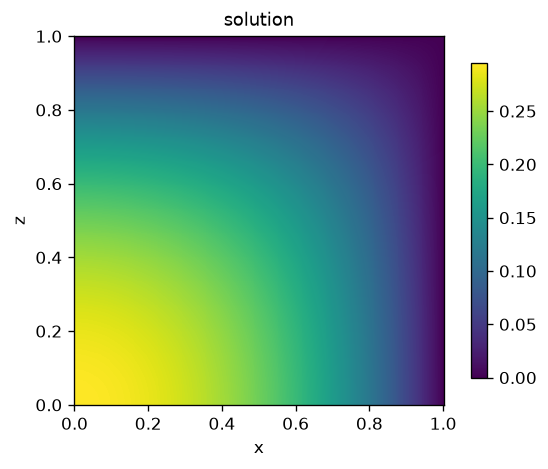
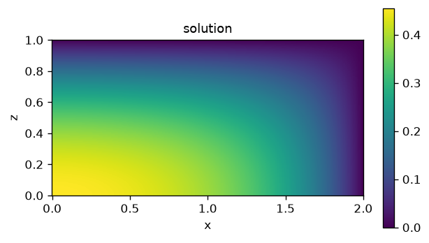
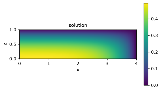
Each is the smooth interior bump of \(\nabla^2 u = -1\): zero on the no-slip (Dirichlet) edges, with the peak flattening and stretching as the domain widens.