Barotropic vorticity on a beta-plane

This example sits on top of the periodic multigrid core: it integrates the barotropic vorticity equation

\[ \frac{\partial \zeta}{\partial t} = -J(\psi, \zeta) - \beta\,\frac{\partial \psi}{\partial x} + D(\zeta), \qquad \nabla^2 \psi = \zeta, \]

on a doubly-periodic square, recovering the streamfunction \(\psi\) from the vorticity \(\zeta\) with a periodic Poisson solve every Runge--Kutta stage. The theory page covers the Arakawa Jacobian, the SSP-RK3 step and the null-space handling; this page drives the API.

Both code blocks below are regions of tests/snippets/vorticity_tutorial.cpp, compiled and run as part of the test suite.

Headers

Unlike the Poisson and Bratu tutorials, the vorticity model is not a mgrid:: class you subclass -- it is a small standalone library (examples/vorticity) with three headers:

#include "../../examples/vorticity/barotropic.hpp"
#include "../../examples/vorticity/diagnostics.hpp"
#include "../../examples/vorticity/initial_conditions.hpp"

barotropic.hpp has the BarotropicVorticity state/stepper, diagnostics.hpp the vdiag:: scalar diagnostics (energy, enstrophy, kurtosis, spectrum), and initial_conditions.hpp the vic:: initial-vorticity fields.

Set up and run

    // 64x64 doubly-periodic torus, beta-plane, weak biharmonic hyperviscosity.
    BarotropicVorticity model(/*numberOfGrids=*/4, /*minimumResolution=*/8,
                              /*beta=*/1.0, /*nu=*/1e-14, /*dissipationOrder=*/2);

    mgrid::Field2D z(model.nx(), model.nz());
    vic::random_peaked_spectrum(z, /*k0=*/6.0, /*seed=*/1u, 1.0, 1.0);
    model.set_zeta(z);

    mgrid::Field2D rhs(model.nx(), model.nz());
    model.rhs(model.zeta(), rhs); // one inversion to populate psi
    const double e0 = vdiag::energy(model.psi(), model.zeta());

    for (int step = 0; step < 50; ++step)
        model.step(0.4 * model.cfl_dt());

    model.rhs(model.zeta(), rhs);
    const double e1 = vdiag::energy(model.psi(), model.zeta());

The constructor arguments are, in order:

numberOfGrids = 4, minimumResolution = 8 -- the periodic multigrid hierarchy. The finest grid is minimumResolution * 2^(numberOfGrids - 1) = \(64\) points per axis; minimumResolution must be even.
beta = 1.0 -- the planetary-vorticity gradient. Non-zero here, so the flow carries Rossby waves as well as turbulence.
nu = 1e-14, dissipationOrder = 2 -- weak biharmonic hyperviscosity, a small-scale sink that keeps the enstrophy cascade from piling up at the grid scale without noticeably damping the large eddies.

vic::random_peaked_spectrum fills z with a random field whose kinetic-energy spectrum peaks near shell k0 = 6 -- a McWilliams-style decaying-turbulence initial condition, deterministic for a fixed seed. set_zeta stores it and projects out its mean so the periodic Poisson solve stays well posed.

rhs(zeta, out) evaluates the tendency, and as a side effect inverts \(\nabla^2\psi = \zeta\) so that psi() matches the current zeta(). That call is needed before every diagnostic read: energy wants a \(\psi\)/\(\zeta\) pair that actually solves the Poisson equation, and step() leaves psi() about one step stale (it holds the last Runge--Kutta stage's streamfunction). Hence the rhs call before e0, and again after the loop before e1.

cfl_dt() returns the advective CFL step from the most recent \(\psi\); the loop takes a further \(0.4\times\) safety margin on top of its default factor. After 50 steps the test checks that the energy is finite and that e1 / e0 > 0.5 -- a loose sanity bound that fails loudly if the scheme goes unstable or the solve collapses, without pinning a number that depends on the RNG.

Running the full example

The built binary runs longer integrations and writes fields to disk:

./build/examples/vorticity/vorticity --case spectral --n 128 --steps 2000 \
    --snapshot-every 200 --out ./

This takes a little over two minutes on the dev container. It runs with the default biharmonic hyperviscosity --nu 1.3e-9 (--dissipation-order 2), which is the spectral regression test's nu = 4e-9 at N = 96 rescaled to N = 128 by the h^4 biharmonic-damping law -- strong enough that the enstrophy cascade dissipates at the grid scale instead of piling up. Over the run you should see the energy hold to within a few percent, the enstrophy fall by roughly 70 %, and the vorticity kurtosis climb from ~2.8 past 6 as coherent vortices emerge (it first crosses 5 near step 1600). A far smaller --nu leaves the run effectively inviscid at this resolution and none of that happens.

--case selects the preset: rossby (a single small-amplitude Rossby wave, beta honoured), conservation (white-noise vorticity, beta forced to 0), or spectral (the peaked-spectrum turbulence run, beta forced to 0). --n must be even with n / 8 a power of two. Other flags: --aspect, --beta, --nu, --dissipation-order, and --help.

Every --snapshot-every steps (and at step 0 and the last step) the run writes vorticity_<case>_<step>.nc, a netCDF file holding the 2-D zeta and psi fields plus time, energy and enstrophy global attributes. In parallel it prints a CSV table to stdout with columns step,time,energy,enstrophy,vorticity_kurtosis -- enough to plot the invariants and watch the kurtosis climb as coherent vortices emerge.

Visualising the results

The spectral run above (just viz-data then just viz) renders the final snapshot and the diagnostics table:

Final zeta and psi snapshot

Energy, enstrophy and vorticity kurtosis versus time

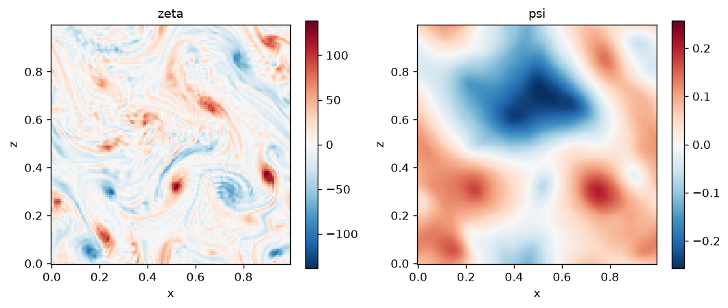
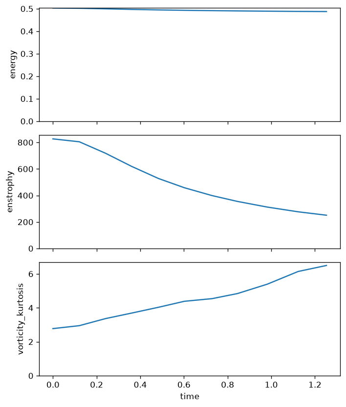
The vorticity field has organised into a few coherent same-sign vortices; the streamfunction is correspondingly smooth and large-scale. The diagnostics show the signature of freely decaying 2-D turbulence: energy nearly conserved, the enstrophy decaying sharply, and the vorticity kurtosis climbing well past its Gaussian value of 3 as the vortices emerge.